Matched mouse cortex data expeirment
Step 1: Data preprocessing
Here, we will guide you through the process of preparing the required data for scCross model training.
[1]:
import anndata
import networkx as nx
import scanpy as sc
import sccross
import pandas as pd
import seaborn as sns
from matplotlib import rcParams
[2]:
rcParams["figure.figsize"] = (4, 4)
In this section, we’ll load existing h5ad files, which is the native file format for AnnData. These h5ad files are used for our tutorial and can be downloaded from the following location:
[3]:
rna = anndata.read_h5ad("matched_mouse_cortex_RNA.h5ad")
rna
[3]:
AnnData object with n_obs × n_vars = 9190 × 28930
    obs: 'domain', 'cell_type'
[4]:
atac = anndata.read_h5ad("matched_mouse_cortex_ATAC.h5ad")
atac
[4]:
AnnData object with n_obs × n_vars = 9190 × 241757
    obs: 'domain', 'cell_type'
Preprocess scRNA-seq data
[5]:
rna.layers["counts"] = rna.X.copy()
[6]:
sc.pp.highly_variable_genes(rna, n_top_genes=2000, flavor="seurat_v3")
[7]:
sc.pp.normalize_total(rna)
sc.pp.log1p(rna)
sc.pp.scale(rna)
sc.tl.pca(rna, n_comps=100, svd_solver="auto")
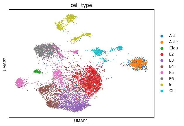
We can visualize the scRNA-seq with UMAP.
[8]:
sc.pp.neighbors(rna, metric="cosine")
sc.tl.umap(rna)
sc.pl.umap(rna, color="cell_type")

Preprocess scATAC-seq data
[10]:
sccross.data.lsi(atac, n_components=100, n_iter=15)
We may also visualize the ATAC domain with UMAP.
[11]:
sc.pp.neighbors(atac, use_rep="X_lsi", metric="cosine")
sc.tl.umap(atac)
sc.pl.umap(atac, color="cell_type")

Prepare atac data’s gene activity score
To calculate the gene activity score for scATAC-seq data based on its peak features, we have re-implemented the geneactivity function from episcanpy in the sccross.data.geneActivity function.
This process allows us to derive gene activity scores from scATAC-seq data, which can be used for downstream analysis and integration with other omics data. Please make sure the species and the location of the GTF reference file. GTF reference file can be downloaded at GENCODE.
[12]:
atac2rna = sccross.data.geneActivity(atac,gtf_file='./reference/gencode.vM30.annotation.gtf')
Save preprocessed data files
Finally, we save the preprocessed data, for use in the training step.
[13]:
atac.uns['gene'] = atac2rna
rna.write("rna_preprocessed.h5ad", compression="gzip")
atac.write("atac_preprocessed.h5ad", compression="gzip")
Step2: Model traning
Config dataset
Before proceeding with model training, it’s essential to configure the datasets using the sccross.models.configure_dataset function. For each dataset that we aim to integrate, we specify the probabilistic generative model to be employed. In this case, we model the raw counts of both scRNA-seq and scATAC-seq data using the negative binomial distribution ("NB").
Additionally, we have the option to specify whether only highly variable features should be utilized (use_highly_variable), which data layer to use (use_layer), and what preprocessing embedding (use_rep) should be applied as the first encoder transformation.
What’s more, gene set calculation is also performed in this process. Please make sure to copy the gen_sets directory to the main path of you project.
project
|...
└───gene_sets
||c2.cp.v7.4.symbols.gmt
||c5.go.bp.v7.4.symbols.gmt
||Mouse_TF_targets.txt
For the scRNA-seq data, we utilize the raw counts from the “counts” layer and employ the PCA embedding as the initial encoder transformation.
For the scATAC-seq data, the raw counts are directly sourced from
atac.X, making it unnecessary to specify ause_layer. Here, we apply the LSI embedding as the first encoder transformation.
[14]:
sccross.models.configure_dataset(
    rna, "NB", use_highly_variable=True,
    use_layer = 'counts',
     use_rep="X_pca"
)
GMT file c5.go.bp.v7.4.symbols.gmt loading ...
7481
Number of genes in c5.go.bp.v7.4.symbols.gmt 13204
GMT file c2.cp.v7.4.symbols.gmt loading ...
2922
Number of genes in c2.cp.v7.4.symbols.gmt 10362
[15]:
sccross.models.configure_dataset(
    atac, "NB", use_highly_variable=False,
    use_rep="X_lsi"
)
GMT file c5.go.bp.v7.4.symbols.gmt loading ...
7481
Number of genes in c5.go.bp.v7.4.symbols.gmt 0
GMT file c2.cp.v7.4.symbols.gmt loading ...
2922
Number of genes in c2.cp.v7.4.symbols.gmt 0
Config MNN prior
In the sccross.data.mnn_prior function, we begin by identifying the common genes shared between the gene expression data of scRNA-seq and the gene activity score data of scATAC-seq. Using these common features, we apply the MNN (Mutual Nearest Neighbors) algorithm to establish links between cells from different omics datasets.
We leverage an implementation of the MNN correction function provided by Scanpy to reduce the distances between similar cells in different omics datasets. This process yields corrected vectors, which serve as MNN priors for each cell. These MNN priors play a crucial role in subsequent steps for data integration and alignment.
[16]:
sccross.data.mnn_prior([rna,atac])
Train model
Here, we train an sccross model to integrate the omics layers.
[17]:
cross = sccross.models.fit_SCCROSS(
    {"rna": rna, "atac": atac},
    fit_kws={"directory": "sccross"}
)
[INFO] fit_SCCROSS: Pretraining SCCROSS model...
[INFO] autodevice: Using GPU 0 as computation device.
[INFO] SCCROSSModel: Setting `max_epochs` = 372
[INFO] SCCROSSModel: Setting `patience` = 31
[INFO] SCCROSSModel: Setting `reduce_lr_patience` = 16
"[INFO] SCCROSSTrainer: Using training directory: "0929_sccross_oldform_0.04_old_new_10_40/pretrain"\n"[INFO] SCCROSSTrainer: [Epoch 10] train={'x_rna_nll': 0.166, 'x_rna_kl': 0.011, 'x_rna_elbo': 0.177, 'x_atac_nll': 0.039, 'x_atac_kl': 0.005, 'x_atac_elbo': 0.045, 'dsc_loss': 0.0, 'vae_loss': 0.244, 'gen_loss': 0.244}, val={'x_rna_nll': 0.165, 'x_rna_kl': 0.011, 'x_rna_elbo': 0.176, 'x_atac_nll': 0.039, 'x_atac_kl': 0.005, 'x_atac_elbo': 0.045, 'dsc_loss': 0.69, 'vae_loss': 115.492, 'gen_loss': -222.669}, 3.7s elapsed
Epoch    18: reducing learning rate of group 0 to 1.0000e-04.
Epoch    18: reducing learning rate of group 0 to 1.0000e-04.
[INFO] LRScheduler: Learning rate reduction: step 1
[INFO] SCCROSSTrainer: [Epoch 20] train={'x_rna_nll': 0.163, 'x_rna_kl': 0.01, 'x_rna_elbo': 0.173, 'x_atac_nll': 0.039, 'x_atac_kl': 0.005, 'x_atac_elbo': 0.044, 'dsc_loss': 0.0, 'vae_loss': 0.23, 'gen_loss': 0.23}, val={'x_rna_nll': 0.163, 'x_rna_kl': 0.009, 'x_rna_elbo': 0.172, 'x_atac_nll': 0.039, 'x_atac_kl': 0.005, 'x_atac_elbo': 0.044, 'dsc_loss': 0.691, 'vae_loss': 108.591, 'gen_loss': -230.481}, 3.7s elapsed
[INFO] SCCROSSTrainer: [Epoch 30] train={'x_rna_nll': 0.162, 'x_rna_kl': 0.01, 'x_rna_elbo': 0.172, 'x_atac_nll': 0.039, 'x_atac_kl': 0.005, 'x_atac_elbo': 0.044, 'dsc_loss': 0.0, 'vae_loss': 0.229, 'gen_loss': 0.229}, val={'x_rna_nll': 0.166, 'x_rna_kl': 0.009, 'x_rna_elbo': 0.175, 'x_atac_nll': 0.039, 'x_atac_kl': 0.005, 'x_atac_elbo': 0.045, 'dsc_loss': 0.691, 'vae_loss': 110.514, 'gen_loss': -228.592}, 3.7s elapsed
Epoch    35: reducing learning rate of group 0 to 1.0000e-05.
Epoch    35: reducing learning rate of group 0 to 1.0000e-05.
[INFO] LRScheduler: Learning rate reduction: step 2
[INFO] SCCROSSTrainer: [Epoch 40] train={'x_rna_nll': 0.162, 'x_rna_kl': 0.01, 'x_rna_elbo': 0.172, 'x_atac_nll': 0.039, 'x_atac_kl': 0.005, 'x_atac_elbo': 0.044, 'dsc_loss': 0.0, 'vae_loss': 0.229, 'gen_loss': 0.229}, val={'x_rna_nll': 0.164, 'x_rna_kl': 0.009, 'x_rna_elbo': 0.174, 'x_atac_nll': 0.04, 'x_atac_kl': 0.005, 'x_atac_elbo': 0.045, 'dsc_loss': 0.692, 'vae_loss': 109.687, 'gen_loss': -229.268}, 3.7s elapsed
[INFO] SCCROSSTrainer: [Epoch 50] train={'x_rna_nll': 0.162, 'x_rna_kl': 0.01, 'x_rna_elbo': 0.171, 'x_atac_nll': 0.038, 'x_atac_kl': 0.005, 'x_atac_elbo': 0.044, 'dsc_loss': 0.0, 'vae_loss': 0.228, 'gen_loss': 0.228}, val={'x_rna_nll': 0.162, 'x_rna_kl': 0.009, 'x_rna_elbo': 0.172, 'x_atac_nll': 0.04, 'x_atac_kl': 0.005, 'x_atac_elbo': 0.045, 'dsc_loss': 0.692, 'vae_loss': 109.603, 'gen_loss': -229.485}, 3.7s elapsed
Epoch    52: reducing learning rate of group 0 to 1.0000e-06.
Epoch    52: reducing learning rate of group 0 to 1.0000e-06.
[INFO] LRScheduler: Learning rate reduction: step 3
[INFO] SCCROSSTrainer: [Epoch 60] train={'x_rna_nll': 0.162, 'x_rna_kl': 0.01, 'x_rna_elbo': 0.172, 'x_atac_nll': 0.039, 'x_atac_kl': 0.005, 'x_atac_elbo': 0.044, 'dsc_loss': 0.0, 'vae_loss': 0.228, 'gen_loss': 0.228}, val={'x_rna_nll': 0.161, 'x_rna_kl': 0.009, 'x_rna_elbo': 0.171, 'x_atac_nll': 0.039, 'x_atac_kl': 0.005, 'x_atac_elbo': 0.045, 'dsc_loss': 0.692, 'vae_loss': 109.05, 'gen_loss': -230.132}, 3.7s elapsed
Epoch    69: reducing learning rate of group 0 to 1.0000e-07.
Epoch    69: reducing learning rate of group 0 to 1.0000e-07.
[INFO] LRScheduler: Learning rate reduction: step 4
[INFO] SCCROSSTrainer: [Epoch 70] train={'x_rna_nll': 0.162, 'x_rna_kl': 0.01, 'x_rna_elbo': 0.171, 'x_atac_nll': 0.039, 'x_atac_kl': 0.005, 'x_atac_elbo': 0.044, 'dsc_loss': 0.0, 'vae_loss': 0.228, 'gen_loss': 0.228}, val={'x_rna_nll': 0.16, 'x_rna_kl': 0.009, 'x_rna_elbo': 0.169, 'x_atac_nll': 0.04, 'x_atac_kl': 0.005, 'x_atac_elbo': 0.045, 'dsc_loss': 0.691, 'vae_loss': 108.937, 'gen_loss': -230.424}, 3.7s elapsed
[INFO] EarlyStopping: Restoring checkpoint 45...
[INFO] fit_SCCROSS: Fine-tuning SCCROSS model...
[INFO] SCCROSSModel: Setting `align_burnin` = 62
[INFO] SCCROSSModel: Setting `max_epochs` = 372
[INFO] SCCROSSModel: Setting `patience` = 31
[INFO] SCCROSSModel: Setting `reduce_lr_patience` = 16
"[INFO] SCCROSSTrainer: Using training directory: "0929_sccross_oldform_0.04_old_new_10_40/fine-tune"\n"[INFO] SCCROSSTrainer: [Epoch 10] train={'x_rna_nll': 0.164, 'x_rna_kl': 0.012, 'x_rna_elbo': 0.176, 'x_atac_nll': 0.039, 'x_atac_kl': 0.001, 'x_atac_elbo': 0.039, 'dsc_loss': 0.572, 'vae_loss': 4.869, 'gen_loss': -37.522}, val={'x_rna_nll': 0.164, 'x_rna_kl': 0.012, 'x_rna_elbo': 0.176, 'x_atac_nll': 0.04, 'x_atac_kl': 0.001, 'x_atac_elbo': 0.04, 'dsc_loss': 0.552, 'vae_loss': 3.405, 'gen_loss': -1072.07}, 9.9s elapsed
[INFO] SCCROSSTrainer: [Epoch 20] train={'x_rna_nll': 0.163, 'x_rna_kl': 0.012, 'x_rna_elbo': 0.176, 'x_atac_nll': 0.039, 'x_atac_kl': 0.001, 'x_atac_elbo': 0.039, 'dsc_loss': 0.606, 'vae_loss': 4.438, 'gen_loss': -28.224}, val={'x_rna_nll': 0.164, 'x_rna_kl': 0.012, 'x_rna_elbo': 0.176, 'x_atac_nll': 0.039, 'x_atac_kl': 0.001, 'x_atac_elbo': 0.04, 'dsc_loss': 0.624, 'vae_loss': 2.904, 'gen_loss': -1411.128}, 9.8s elapsed
[INFO] SCCROSSTrainer: [Epoch 30] train={'x_rna_nll': 0.163, 'x_rna_kl': 0.012, 'x_rna_elbo': 0.175, 'x_atac_nll': 0.039, 'x_atac_kl': 0.001, 'x_atac_elbo': 0.039, 'dsc_loss': 0.623, 'vae_loss': 4.299, 'gen_loss': -15.061}, val={'x_rna_nll': 0.167, 'x_rna_kl': 0.012, 'x_rna_elbo': 0.179, 'x_atac_nll': 0.04, 'x_atac_kl': 0.001, 'x_atac_elbo': 0.04, 'dsc_loss': 0.624, 'vae_loss': 3.49, 'gen_loss': -1825.241}, 9.9s elapsed
[INFO] SCCROSSTrainer: [Epoch 40] train={'x_rna_nll': 0.163, 'x_rna_kl': 0.012, 'x_rna_elbo': 0.175, 'x_atac_nll': 0.039, 'x_atac_kl': 0.001, 'x_atac_elbo': 0.039, 'dsc_loss': 0.62, 'vae_loss': 4.135, 'gen_loss': -14.574}, val={'x_rna_nll': 0.165, 'x_rna_kl': 0.011, 'x_rna_elbo': 0.176, 'x_atac_nll': 0.04, 'x_atac_kl': 0.001, 'x_atac_elbo': 0.041, 'dsc_loss': 0.627, 'vae_loss': 2.733, 'gen_loss': -1945.286}, 9.9s elapsed
[INFO] SCCROSSTrainer: [Epoch 50] train={'x_rna_nll': 0.162, 'x_rna_kl': 0.012, 'x_rna_elbo': 0.174, 'x_atac_nll': 0.038, 'x_atac_kl': 0.001, 'x_atac_elbo': 0.039, 'dsc_loss': 0.607, 'vae_loss': 4.017, 'gen_loss': -9.334}, val={'x_rna_nll': 0.162, 'x_rna_kl': 0.012, 'x_rna_elbo': 0.174, 'x_atac_nll': 0.04, 'x_atac_kl': 0.001, 'x_atac_elbo': 0.041, 'dsc_loss': 0.623, 'vae_loss': 2.736, 'gen_loss': -2224.985}, 9.9s elapsed
[INFO] SCCROSSTrainer: [Epoch 60] train={'x_rna_nll': 0.162, 'x_rna_kl': 0.011, 'x_rna_elbo': 0.173, 'x_atac_nll': 0.039, 'x_atac_kl': 0.001, 'x_atac_elbo': 0.039, 'dsc_loss': 0.587, 'vae_loss': 3.897, 'gen_loss': -9.616}, val={'x_rna_nll': 0.162, 'x_rna_kl': 0.011, 'x_rna_elbo': 0.173, 'x_atac_nll': 0.04, 'x_atac_kl': 0.001, 'x_atac_elbo': 0.04, 'dsc_loss': 0.647, 'vae_loss': 2.702, 'gen_loss': -2307.811}, 9.9s elapsed
[INFO] SCCROSSTrainer: [Epoch 70] train={'x_rna_nll': 0.162, 'x_rna_kl': 0.011, 'x_rna_elbo': 0.173, 'x_atac_nll': 0.039, 'x_atac_kl': 0.001, 'x_atac_elbo': 0.039, 'dsc_loss': 0.582, 'vae_loss': 3.901, 'gen_loss': -6.097}, val={'x_rna_nll': 0.16, 'x_rna_kl': 0.01, 'x_rna_elbo': 0.171, 'x_atac_nll': 0.04, 'x_atac_kl': 0.001, 'x_atac_elbo': 0.041, 'dsc_loss': 0.615, 'vae_loss': 2.546, 'gen_loss': -2577.006}, 9.4s elapsed
[INFO] SCCROSSTrainer: [Epoch 80] train={'x_rna_nll': 0.162, 'x_rna_kl': 0.011, 'x_rna_elbo': 0.172, 'x_atac_nll': 0.038, 'x_atac_kl': 0.001, 'x_atac_elbo': 0.039, 'dsc_loss': 0.59, 'vae_loss': 3.834, 'gen_loss': -9.214}, val={'x_rna_nll': 0.162, 'x_rna_kl': 0.01, 'x_rna_elbo': 0.172, 'x_atac_nll': 0.04, 'x_atac_kl': 0.001, 'x_atac_elbo': 0.041, 'dsc_loss': 0.646, 'vae_loss': 2.586, 'gen_loss': -2501.872}, 9.3s elapsed
[INFO] SCCROSSTrainer: [Epoch 90] train={'x_rna_nll': 0.161, 'x_rna_kl': 0.011, 'x_rna_elbo': 0.172, 'x_atac_nll': 0.038, 'x_atac_kl': 0.001, 'x_atac_elbo': 0.039, 'dsc_loss': 0.589, 'vae_loss': 3.791, 'gen_loss': -6.109}, val={'x_rna_nll': 0.164, 'x_rna_kl': 0.01, 'x_rna_elbo': 0.174, 'x_atac_nll': 0.04, 'x_atac_kl': 0.001, 'x_atac_elbo': 0.041, 'dsc_loss': 0.619, 'vae_loss': 2.588, 'gen_loss': -2504.729}, 9.4s elapsed
[INFO] SCCROSSTrainer: [Epoch 100] train={'x_rna_nll': 0.162, 'x_rna_kl': 0.01, 'x_rna_elbo': 0.172, 'x_atac_nll': 0.039, 'x_atac_kl': 0.001, 'x_atac_elbo': 0.039, 'dsc_loss': 0.594, 'vae_loss': 3.724, 'gen_loss': -4.537}, val={'x_rna_nll': 0.163, 'x_rna_kl': 0.01, 'x_rna_elbo': 0.173, 'x_atac_nll': 0.04, 'x_atac_kl': 0.001, 'x_atac_elbo': 0.041, 'dsc_loss': 0.584, 'vae_loss': 2.658, 'gen_loss': -2462.062}, 9.4s elapsed
[INFO] SCCROSSTrainer: [Epoch 110] train={'x_rna_nll': 0.162, 'x_rna_kl': 0.01, 'x_rna_elbo': 0.172, 'x_atac_nll': 0.038, 'x_atac_kl': 0.001, 'x_atac_elbo': 0.039, 'dsc_loss': 0.59, 'vae_loss': 3.698, 'gen_loss': -5.915}, val={'x_rna_nll': 0.161, 'x_rna_kl': 0.009, 'x_rna_elbo': 0.171, 'x_atac_nll': 0.04, 'x_atac_kl': 0.001, 'x_atac_elbo': 0.041, 'dsc_loss': 0.611, 'vae_loss': 2.53, 'gen_loss': -2511.721}, 9.4s elapsed
[INFO] SCCROSSTrainer: [Epoch 120] train={'x_rna_nll': 0.161, 'x_rna_kl': 0.01, 'x_rna_elbo': 0.171, 'x_atac_nll': 0.038, 'x_atac_kl': 0.001, 'x_atac_elbo': 0.039, 'dsc_loss': 0.59, 'vae_loss': 3.632, 'gen_loss': -5.581}, val={'x_rna_nll': 0.163, 'x_rna_kl': 0.009, 'x_rna_elbo': 0.173, 'x_atac_nll': 0.04, 'x_atac_kl': 0.001, 'x_atac_elbo': 0.041, 'dsc_loss': 0.603, 'vae_loss': 2.409, 'gen_loss': -2838.794}, 9.4s elapsed
Epoch   125: reducing learning rate of group 0 to 1.0000e-04.
Epoch   125: reducing learning rate of group 0 to 1.0000e-04.
[INFO] LRScheduler: Learning rate reduction: step 1
[INFO] SCCROSSTrainer: [Epoch 130] train={'x_rna_nll': 0.162, 'x_rna_kl': 0.009, 'x_rna_elbo': 0.172, 'x_atac_nll': 0.038, 'x_atac_kl': 0.001, 'x_atac_elbo': 0.039, 'dsc_loss': 0.608, 'vae_loss': 3.37, 'gen_loss': -0.567}, val={'x_rna_nll': 0.162, 'x_rna_kl': 0.009, 'x_rna_elbo': 0.171, 'x_atac_nll': 0.04, 'x_atac_kl': 0.001, 'x_atac_elbo': 0.04, 'dsc_loss': 0.616, 'vae_loss': 2.3, 'gen_loss': -2862.844}, 9.5s elapsed
[INFO] SCCROSSTrainer: [Epoch 140] train={'x_rna_nll': 0.161, 'x_rna_kl': 0.009, 'x_rna_elbo': 0.171, 'x_atac_nll': 0.038, 'x_atac_kl': 0.001, 'x_atac_elbo': 0.039, 'dsc_loss': 0.609, 'vae_loss': 3.369, 'gen_loss': -0.149}, val={'x_rna_nll': 0.161, 'x_rna_kl': 0.009, 'x_rna_elbo': 0.17, 'x_atac_nll': 0.04, 'x_atac_kl': 0.001, 'x_atac_elbo': 0.041, 'dsc_loss': 0.599, 'vae_loss': 2.226, 'gen_loss': -3001.546}, 9.4s elapsed
[INFO] SCCROSSTrainer: [Epoch 150] train={'x_rna_nll': 0.162, 'x_rna_kl': 0.009, 'x_rna_elbo': 0.171, 'x_atac_nll': 0.038, 'x_atac_kl': 0.001, 'x_atac_elbo': 0.039, 'dsc_loss': 0.609, 'vae_loss': 3.328, 'gen_loss': 0.078}, val={'x_rna_nll': 0.16, 'x_rna_kl': 0.009, 'x_rna_elbo': 0.169, 'x_atac_nll': 0.04, 'x_atac_kl': 0.001, 'x_atac_elbo': 0.04, 'dsc_loss': 0.596, 'vae_loss': 2.265, 'gen_loss': -3052.171}, 9.4s elapsed
Epoch   157: reducing learning rate of group 0 to 1.0000e-05.
Epoch   157: reducing learning rate of group 0 to 1.0000e-05.
[INFO] LRScheduler: Learning rate reduction: step 2
[INFO] SCCROSSTrainer: [Epoch 160] train={'x_rna_nll': 0.161, 'x_rna_kl': 0.009, 'x_rna_elbo': 0.171, 'x_atac_nll': 0.039, 'x_atac_kl': 0.001, 'x_atac_elbo': 0.039, 'dsc_loss': 0.61, 'vae_loss': 3.325, 'gen_loss': 0.394}, val={'x_rna_nll': 0.16, 'x_rna_kl': 0.009, 'x_rna_elbo': 0.169, 'x_atac_nll': 0.04, 'x_atac_kl': 0.001, 'x_atac_elbo': 0.04, 'dsc_loss': 0.599, 'vae_loss': 2.248, 'gen_loss': -3079.63}, 9.3s elapsed
[INFO] SCCROSSTrainer: [Epoch 170] train={'x_rna_nll': 0.161, 'x_rna_kl': 0.009, 'x_rna_elbo': 0.171, 'x_atac_nll': 0.038, 'x_atac_kl': 0.001, 'x_atac_elbo': 0.039, 'dsc_loss': 0.615, 'vae_loss': 3.33, 'gen_loss': 0.639}, val={'x_rna_nll': 0.162, 'x_rna_kl': 0.009, 'x_rna_elbo': 0.171, 'x_atac_nll': 0.04, 'x_atac_kl': 0.001, 'x_atac_elbo': 0.04, 'dsc_loss': 0.586, 'vae_loss': 2.332, 'gen_loss': -3129.936}, 9.3s elapsed
[INFO] SCCROSSTrainer: [Epoch 180] train={'x_rna_nll': 0.161, 'x_rna_kl': 0.009, 'x_rna_elbo': 0.17, 'x_atac_nll': 0.039, 'x_atac_kl': 0.001, 'x_atac_elbo': 0.039, 'dsc_loss': 0.61, 'vae_loss': 3.308, 'gen_loss': 0.34}, val={'x_rna_nll': 0.161, 'x_rna_kl': 0.009, 'x_rna_elbo': 0.17, 'x_atac_nll': 0.04, 'x_atac_kl': 0.001, 'x_atac_elbo': 0.041, 'dsc_loss': 0.59, 'vae_loss': 2.392, 'gen_loss': -3167.259}, 9.5s elapsed
Epoch   182: reducing learning rate of group 0 to 1.0000e-06.
Epoch   182: reducing learning rate of group 0 to 1.0000e-06.
[INFO] LRScheduler: Learning rate reduction: step 3
[INFO] SCCROSSTrainer: [Epoch 190] train={'x_rna_nll': 0.162, 'x_rna_kl': 0.009, 'x_rna_elbo': 0.171, 'x_atac_nll': 0.038, 'x_atac_kl': 0.001, 'x_atac_elbo': 0.039, 'dsc_loss': 0.608, 'vae_loss': 3.335, 'gen_loss': 0.415}, val={'x_rna_nll': 0.161, 'x_rna_kl': 0.009, 'x_rna_elbo': 0.17, 'x_atac_nll': 0.04, 'x_atac_kl': 0.001, 'x_atac_elbo': 0.041, 'dsc_loss': 0.597, 'vae_loss': 2.307, 'gen_loss': -3147.56}, 9.3s elapsed
[INFO] EarlyStopping: Restoring checkpoint 171...
After training, the trained model can be saved and loaded as “.dill” files. The trained model can be found in the following location:
[18]:
cross.save("matched_mouse_cortex.dill")
#cross = sccross.models.load_model("matched_mouse_cortex.dill")
Step3: Single cell multi-omics integration
After training the model, we can utilize the encode_data method to project the single-cell omics data into integrated cell embeddings.
The first argument of encode_data specifies the domain for encoding, which should correspond to one of the previously defined domain names.
The second argument specifies the dataset to be encoded.
As a convention, we store the resulting cell embeddings in the obsm slot, with the name "X_cross".
[19]:
rna.obsm["X_cross"] = cross.encode_data("rna", rna)
atac.obsm["X_cross"] = cross.encode_data("atac", atac)
To jointly visualize the cell embeddings from two omics layers, we construct a combined dataset.
[20]:
combined = anndata.concat([rna, atac])
Then we use UMAP to visualize the aligned embeddings. We can see that the two omics layers are now correctly aligned.
[21]:
sc.pp.neighbors(combined, use_rep="X_cross", metric="cosine")
sc.tl.umap(combined)
sc.pl.umap(combined, color=["cell_type", "domain"], wspace=0.65)

Step4: Single cell multi-omics cross modality generation
To achieve cross-modality data generation, we have the generate_cross function at our disposal. Using this function, we can seamlessly transfer data from one modality to another, even when the modalities are not matched.
The key information is placed in the first position, while the data to be generated is positioned in the third position.
The function also requires the training data of a specific modality to be provided in the remaining positions. This ensures that the generated data closely follows the scale and distribution of the real data from the training set.
By using generate_cross, we can perform cross-modality data generation effectively and maintain data fidelity.
[22]:
atacCrorna = cross.generate_cross( 'atac', 'rna', atac, rna)
atacCrorna = sc.AnnData(atacCrorna,obs=atac.obs,var= rna.var.query("highly_variable"))
Then we can process the generated data and use UMAP to visualize the cross generation result.
[23]:
sc.pp.normalize_total(atacCrorna)
sc.pp.log1p(atacCrorna)
sc.pp.scale(atacCrorna)
sc.tl.pca(atacCrorna, n_comps=100, svd_solver="auto")
sc.pp.neighbors(atacCrorna,  metric="cosine")
sc.tl.umap(atacCrorna)
sc.pl.umap(atacCrorna, color=["cell_type"])

Step5: Single cell omics data self augmentation
In our toolkit, we have the generat_augment function. It is designed to leverage the complementary information present in different omics data types. Each omics dataset can augment its performance in bio-analysis by learning from and integrating information from other omics.
[24]:
rna.obsm['augmented'] = cross.generate_augment( 'rna', rna)
Subsequently, we can identify key differential genes within the augmented scRNA-seq data. It’s important to note that if we train our model with use_highly_variable set to True during the data configuration, the output will exclusively contain highly variable genes. These highly variable genes are often of particular interest in bio-analysis due to their potential significance.
[25]:
rna_augmented = sc.AnnData(rna.obsm['augmented'],obs=rna.obs,var = rna.var.query("highly_variable"))
sc.pp.normalize_total(rna_augmented)
sc.pp.log1p(rna_augmented)
sc.pp.scale(rna_augmented)
sc.tl.rank_genes_groups(rna_augmented,'cell_type')
df = pd.DataFrame(rna_augmented.uns['rank_genes_groups']['names'])
df.to_csv('rna_augmented_rankGenes_cellType.csv')
Step6: Single cell multi-omics matched simulation
Our model offers the capability to perform single-cell multi-omics matched simulation through the generate_multiSim function. This function empowers us to generate matched multi-omics simulated data with flexibility in terms of the number of omics modalities, the cell states, and the number of cells.
To achieve this, we need to specify the following:
The data sources we wish to generate simultaneously.
The observation key associated with the simulated data.
The cluster names to be included in the simulation.
The desired number of cells for the simulation.
With these parameters, we can create matched multi-omics simulated data tailored to our specific requirements.
[26]:
multi_simu = cross.generate_multiSim({'rna':rna,'atac':atac},'cell_type','Ast',len(rna[rna.obs['cell_type'].isin(['Ast'])]))
for adata in multi_simu:
    adata.obs['cell_type'] = 'Ast_s'
We can concate the simulated data with the original data.
[27]:
rna_temp = rna.copy()
rna_temp.X = rna_temp.layers['counts']
rna_temp = rna_temp[:,rna_temp.var.query("highly_variable").index]
rna_temp = sc.concat([rna_temp,multi_simu[0]])
[28]:
atac_temp = atac.copy()
atac_temp = atac_temp[:,atac_temp.var.query("highly_variable").index]
atac_temp = sc.concat([atac_temp,multi_simu[1]])
Then we can process and draw UMAP for the simulated data.
[29]:
sc.pp.normalize_total(rna_temp)
sc.pp.log1p(rna_temp)
sc.pp.scale(rna_temp)
sc.tl.pca(rna_temp, n_comps=100, svd_solver="auto")
sc.pp.neighbors(rna_temp,  metric="cosine")
sc.tl.umap(rna_temp)
sc.pl.umap(rna_temp, color=["cell_type"])
[30]:
sccross.data.lsi(atac_temp, n_components=100, n_iter=15)
sc.pp.neighbors(atac_temp, use_rep = 'X_lsi',  metric="cosine")
sc.tl.umap(atac_temp)
sc.pl.umap(atac_temp, color=["cell_type"])

Step7: Single cell multi-omics in-silico perturbation
Identify genes’ differential expression between cell clusters with in-silico perturbation
For the purpose of identifying differential gene expression between cell clusters, we have developed the perturbation_difGenes function. This function serves as a valuable tool for assessing the importance of genes by measuring the movement of latent expression between cell clusters during in-silico perturbations of the input data.
In order to utilize this function effectively, you need to specify the following:
The modality’s key that corresponds to the target data.
The actual modality’s data.
The observation key associated with the perturbation cell clusters.
The reference cell cluster for comparison.
The genes you intend to perturb within the analysis.
With these parameters, you can gain insights into the differential gene expression patterns between cell clusters and assess the impact of gene perturbations on the latent expression profiles.
[31]:
import random
rna.X = rna.layers['counts']
genes = random.sample(rna.var.query("highly_variable").index.to_numpy().tolist(),100)
difGenes = cross.perturbation_difGenes('rna',rna,'cell_type','Clau','Ast',genes)
difGenes.to_csv('difGens.csv')
The bigger the number in the table means more close to the reference after the up or down perturbated.
[32]:
difGenes
[32]:
| up | down | |
|---|---|---|
| 0 | Shisa6 | Ppfibp2 |
| 1 | Galnt18 | Ighm |
| 2 | 9530026P05Rik | Nefl |
| 3 | Caln1 | Fra10ac1 |
| 4 | Cntnap5a | 9330171B17Rik |
| ... | ... | ... |
| 95 | Pir | Cacna2d2 |
| 96 | Atp13a5 | Unc13c |
| 97 | Platr14 | Vmac |
| 98 | Unc13c | Rgs12 |
| 99 | Cacng4 | Cacng4 |
100 rows × 2 columns
Maintain in-silico perturbation while cross generation
A noteworthy capability of our model is its ability to preserve in-silico perturbations made within one modality while transitioning them to another through cross-modality generation. This means that perturbations initiated in one modality can be seamlessly transferred and observed in another, enabling a cohesive exploration of perturbation effects and responses across different modalities. Here, for fair, we randomly select 100 genes in high variable genes to perform the experiment as an example.
[33]:
rna[rna.obs['cell_type'].isin(['Clau']),difGenes['up'][:100]].X += 0.5*rna[rna.obs['cell_type'].isin(['Clau']),difGenes['up'][:100]].X
rnaCroatac = cross.generate_cross( 'rna', 'atac', rna, atac)
rnaCroatac = sc.AnnData(rnaCroatac,obs=rna.obs,var= atac.var.query("highly_variable"))
rnaCroatac
[33]:
AnnData object with n_obs × n_vars = 9190 × 241757
    obs: 'domain', 'cell_type'